
Dimensionality Reduction
High-dimensional molecular embeddings, while rich in information, are difficult to visualize and interpret directly. The Dimensionality Reduction module in ChemXploreML provides a suite of powerful algorithms to project these embeddings into a lower-dimensional space (typically 2D or 3D), making it possible to visualize the chemical space, identify clusters, and understand the relationships between molecules.
Overview
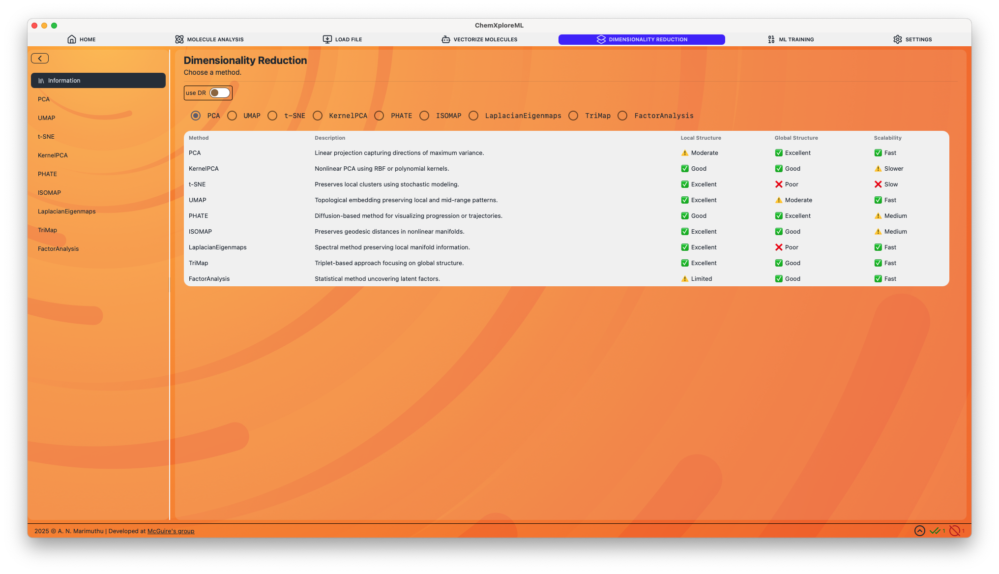
Workflow
The process of applying dimensionality reduction involves the following steps:
- Select Embedder: Choose the molecular embedding that you want to reduce. These are the embeddings you generated in the "Embed Molecule" section.
- Choose a Method: Select a dimensionality reduction algorithm from the available tabs. Each method has its own strengths and is suited for different types of analysis.
- Configure Parameters: Adjust the parameters for the selected algorithm. You can hover over each parameter to get a description of what it does.
- Save Parameters: Before running the reduction, you must save your parameter configuration. This creates a reusable settings file and ensures your workflow is reproducible.
- Run Reduction: Click the "Run" button to start the dimensionality reduction process. The application will save the resulting low-dimensional embeddings as a new
.npyfile. - Visualize: The reduced embeddings can then be used for visualization and further analysis.
Supported Methods
Below is a detailed description of each supported dimensionality reduction method and its configurable parameters.
PCA (Principal Component Analysis)
- Description: A linear technique that transforms the data into a new coordinate system, where the axes (principal components) are orthogonal and capture the maximum variance in the data.
- Local Structure: ⚠️ Moderate
- Global Structure: ✅ Excellent
- Scalability: ✅ Fast
Parameters:
n_components: The number of principal components to keep. Default: 70.random_state: Seed for the random number generator. Default: 42.
UMAP (Uniform Manifold Approximation and Projection)
- Description: A non-linear technique excellent for preserving both local and some global structure. It is often used for visualizing clusters in high-dimensional data.
- Local Structure: ✅ Excellent
- Global Structure: ⚠️ Moderate
- Scalability: ✅ Fast
Parameters:
n_neighbors: Controls how UMAP balances local versus global structure. Default: 15.min_dist: The minimum distance between embedded points. Default: 0.1.n_components: The dimension of the space to embed into. Default: 2.metric: The distance metric to use. Default: 'euclidean'.random_state: Seed for the random number generator. Default: 42.
t-SNE (t-Distributed Stochastic Neighbor Embedding)
- Description: A non-linear technique that is particularly good at revealing the underlying cluster structure in the data. It excels at preserving local structure.
- Local Structure: ✅ Excellent
- Global Structure: ❌ Poor
- Scalability: ❌ Slow
Parameters:
n_components: The dimension of the space to embed into. Default: 2.perplexity: Related to the number of nearest neighbors considered for each point. Default: 30.random_state: Seed for the random number generator. Default: 42.
KernelPCA
- Description: An extension of PCA that uses kernel methods to perform non-linear dimensionality reduction.
- Local Structure: ✅ Good
- Global Structure: ✅ Good
- Scalability: ⚠️ Slower
Parameters:
n_components: Number of components to keep. Default: 2.kernel: The kernel function to use ('linear', 'poly', 'rbf', 'sigmoid', 'cosine'). Default: 'rbf'.gamma: Kernel coefficient. Default: null.
PHATE (Potential of Heat-diffusion for Affinity-based Trajectory Embedding)
- Description: A visualization method that captures both local and global nonlinear structure using a heat-diffusion-based affinity metric. It is particularly well-suited for visualizing trajectories and progressions in data.
- Local Structure: ✅ Good
- Global Structure: ✅ Excellent
- Scalability: ⚠️ Medium
Parameters:
n_components: Number of dimensions to reduce to. Default: 2.knn: Number of nearest neighbors. Default: 5.decay: Controls the decay of the kernel. Default: 40.t: Diffusion time scale. Default: 'auto'.random_state: Seed for reproducibility. Default: 42.
ISOMAP
- Description: A non-linear technique that preserves the geodesic distances between points on a manifold.
- Local Structure: ✅ Excellent
- Global Structure: ✅ Good
- Scalability: ⚠️ Medium
Parameters:
n_components: Number of coordinates for the manifold. Default: 2.n_neighbors: Number of neighbors to consider for each point. Default: 5.
Laplacian Eigenmaps
- Description: A spectral method that preserves local manifold information by constructing a graph from the data and embedding it in a lower-dimensional space.
- Local Structure: ✅ Excellent
- Global Structure: ❌ Poor
- Scalability: ✅ Fast
Parameters:
n_components: Dimension of the embedding space. Default: 2.n_neighbors: Number of neighbors for constructing the neighborhood graph. Default: 10.
TriMap
- Description: A non-linear method that uses triplet constraints to preserve both local and global structure in the data.
- Local Structure: ✅ Excellent
- Global Structure: ✅ Good
- Scalability: ✅ Fast
Parameters:
n_dims: Output dimensionality. Default: 2.n_inliers: Number of inlier points per triplet. Default: 10.n_outliers: Number of outlier points per triplet. Default: 5.n_random: Number of random triplets per point. Default: 5.distance: The distance metric to use. Default: 'euclidean'.
Factor Analysis
- Description: A linear statistical method used to describe variability among observed, correlated variables in terms of a potentially lower number of unobserved variables called factors.
- Local Structure: ⚠️ Limited
- Global Structure: ✅ Good
- Scalability: ✅ Fast
Parameters:
n_components: Number of latent factors to extract. Default: 2.
Next Steps
After reducing the dimensionality of your embeddings, you can:
- Use the 2D or 3D embeddings to create scatter plots and visualize your chemical space.
- Use the reduced-dimension embeddings as features for training a machine learning model.