Machine Learning Training
The Machine Learning Training module is the core of ChemXploreML, providing a comprehensive suite of tools for building, optimizing, and evaluating predictive models for molecular properties. The interface is organized into two main tabs: ML Model for training and ML Prediction for using a trained model.
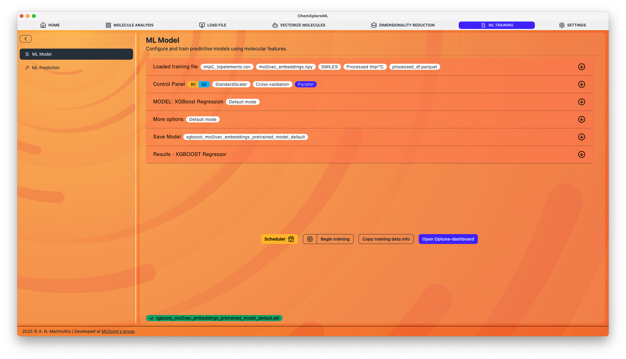
ML Model Tab
This tab contains a multi-panel interface that guides you through the entire model training workflow, from data selection to advanced hyperparameter tuning and model evaluation.
Workflow Overview
- Select Input Data: Choose the molecular embeddings and the corresponding data file.
- Configure Training: Set up the train/test split, cross-validation, and other basic parameters.
- Choose a Model: Select a machine learning algorithm and configure its parameters.
- Set Advanced Options: Optionally, configure advanced features like data cleaning, hyperparameter tuning, and model interpretability analysis.
- Save and Run: Specify a location to save the trained model and its results, then start the training process.
- Analyze Results: Review the performance metrics, plots, and analysis results to evaluate your model.
1. Training File Panel
This panel is for selecting the input data for model training.
- Embeddings File: Choose the
.npyfile containing the molecular embeddings you generated previously. - Training Data File: Select the corresponding data file (e.g., CSV) that contains the target property values (Y-column).
2. Control Panel
Here, you configure the fundamental aspects of the training and validation process.
- Train/Test Split: Set the percentage of data to be used for the test set.
- Cross-Validation: Enable k-fold cross-validation and specify the number of folds. This is highly recommended for robust model evaluation.
- Hyperparameter Tuning: Choose a strategy for optimizing your model's hyperparameters:
- None: Train the model with the manually specified parameters.
- Grid Search: Exhaustively search over a specified subset of the hyperparameter space.
- Randomized Grid Search: Samples a fixed number of parameter settings from the specified distributions.
- Halving Grid Search: An efficient method that successively prunes underperforming parameter combinations.
- Optuna: A powerful Bayesian optimization framework that intelligently searches for the best hyperparameters. You can monitor Optuna's progress using the built-in dashboard.
3. Model Panel
Select the machine learning algorithm and configure its parameters.
- Model: Choose from a wide range of models, including:
- Linear Models: Linear Regression, Ridge, Lasso, ElasticNet
- Support Vector Machines: SVR
- Neighbors: KNN
- Gaussian Process: GPR
- Ensemble Methods: Random Forest (RFR), Gradient Boosting (GBR)
- Advanced Gradient Boosting: XGBoost, LightGBM, CatBoost
- Parameters: For each model, you can manually set its parameters or define a search space for hyperparameter tuning.
4. More Options Panel
This panel contains advanced features for improving your model and gaining deeper insights.
- Y-Transformation and Scaling: Apply transformations (e.g., log, Box-Cox, Yeo-Johnson) and scaling (e.g., StandardScaler, MinMaxScaler) to the target variable. This can be very effective for models that assume a normal distribution of the target.
- Data Augmentation:
- Bootstrap: Create a larger training set by resampling the existing data with replacement.
- Noise Injection: Add random noise to the target variable in the bootstrapped samples to improve model robustness.
- Cleanlab: Use the Cleanlab algorithm to automatically detect and remove mislabeled data points from your dataset before training.
- Learning Curve: Generate a learning curve plot to diagnose whether your model is suffering from high bias or high variance.
- SHAP Analysis: Compute SHAP (SHapley Additive exPlanations) values to understand the importance of each feature in the model's predictions.
5. Save Model and Run
- Save Pretrained Model: Specify a name and location to save your trained model (
.pklfile) and all associated results (plots, metrics, etc.). - Begin Training: Click this button to start the training process. You can monitor the progress in the application's console.
6. Results Panel
After training is complete, this panel will populate with a comprehensive summary of your model's performance.
- Metrics: View key metrics like R², MSE, RMSE, and MAE for both the training and test sets.
- Plots: Analyze the parity plot (predicted vs. actual values) and other visualizations.
- Applicability Domain: Review the leverage and Mahalanobis distance plots to assess whether your model is making reliable predictions.
ML Prediction Tab
Once you have a trained model, you can use the ML Prediction tab to predict the properties of new, unseen molecules.
- Load Model: Select the
.pklfile of your saved model. - Provide Input: Load a file containing the SMILES strings of the molecules you want to predict.
- Run Prediction: The application will generate embeddings for the new molecules and use the loaded model to predict the target property.
- View and Save Results: The predictions will be displayed and can be saved to a file.